optimizer

GPT-2 layer를 구현한 이후에, 실제 학습을 위한 optimizer 구현

You will further implement the step() function of the Adam Optimizer based on Decoupled Weight Decay Regularization and Adam: A Method for Stochastic Optimization in order to train a sentiment classifier.

Decoupled Weight Decay Regularization 및 Adam: A Method for Stochastic Optimization에 기반해서 AdamW optimizer를 직접 구현

Adam Optimzer

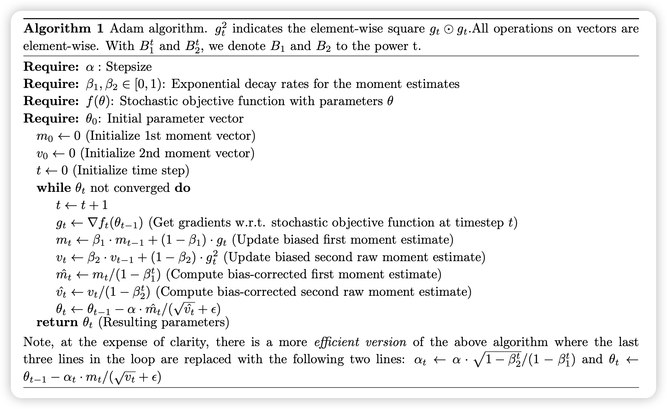
Adam은 SGD 기반의 옵티마이저로, 각각의 파라미터에 대해 1차 모멘트(mean)와 2차 모멘트(variance) 를 유지하면서 learning rate을 adapctive하게 조절해주는 방식 RMSProp과 Momentum의 장점을 모두 가져온 방식으로 널리 사용

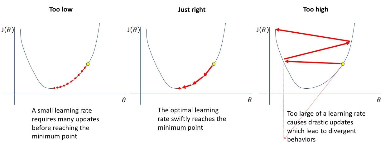
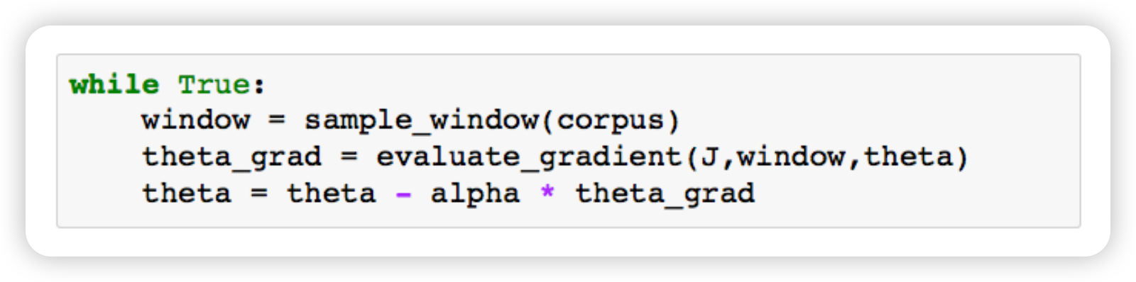
SGD(Stochastic Gradient Descent) 전체 데이터 대신, 미니배치 또는 한 샘플을 기반으로 매번 파라미터를 업데이트 → 실제 학습할 corpus는 너무 많아서 언어모델에선 샘플링 방식으로 해결함

• 1차 모멘트: m_t ← gradient의 지수이동평균
• 2차 모멘트: v_t ← gradient 제곱의 지수이동평균
• 이 두 가지를 통해 parameter update 시 안정성 향상

기존 optimizer와 차이

AdamW는 기존 Adam과 달리 weight decay를 gradient에 포함시키지 않고, 파라미터 업데이트 이후 직접 decay시키는 구조

• Adam: grad ← grad + weight_decay * param 방식 → L2 Regularization처럼 작동
• AdamW: param ← param - lr * weight_decay * param 방식 → Decoupled 방식

⇒ weight decay를 옵티마이저 내부적으로 “분리해서 처리”함으로써 성능 안정성을 향상

구현

def step(self, closure: Callable = None):
        loss = None
        if closure is not None:
            loss = closure()
 
        for group in self.param_groups:
            for p in group["params"]:
                if p.grad is None:
                    continue
                grad = p.grad.data
                if grad.is_sparse:
                    raise RuntimeError("Adam does not support sparse gradients, please consider SparseAdam instead")
 
                # State should be stored in this dictionary.
                state = self.state[p]
 
                # Access hyperparameters from the `group` dictionary.
                alpha = group["lr"]
 
 
                ### TODO: Complete the implementation of AdamW here, reading and saving
                ###       your state in the `state` dictionary above.
                ###       The hyperparameters can be read from the `group` dictionary
                ###       (they are lr, betas, eps, weight_decay, as saved in the constructor).
                ###
                ###       To complete this implementation:
                ###       1. Update the first and second moments of the gradients.
                ###       2. Apply bias correction
                ###          (using the "efficient version" given in https://arxiv.org/abs/1412.6980;
                ###          also given in the pseudo-code in the project description).
                ###       3. Update parameters (p.data).
                ###       4. Apply weight decay after the main gradient-based updates.
                ###
                ###       Refer to the default project handout for more details.
                ### YOUR CODE HERE
 
                beta1, beta2 = group["betas"]
                eps = group["eps"]
                weight_decay = group["weight_decay"]
                correct_bias = group["correct_bias"]
 
				# 시작 단계 상태 초기화
                if len(state) == 0:
                    state["step"] = 0
                    state["exp_avg"] = torch.zeros_like(p.data) 
                    state["exp_avg_sq"] = torch.zeros_like(p.data)
 
                exp_avg = state["exp_avg"] # m_t
                exp_avg_sq = state["exp_avg_sq"] # v_t
 
                state["step"] += 1
                step = state["step"]
 
                # 1차 모멘트
                exp_avg.mul_(beta1).add_(grad, alpha=1 - beta1)
 
                # 2차 모멘트
                exp_avg_sq.mul_(beta2).addcmul_(grad, grad, value=1 - beta2)
 
                # Bias correction
                if correct_bias:
                    bias_correction1 = 1 - beta1 ** step
                    bias_correction2 = 1 - beta2 ** step
                    step_size = alpha * math.sqrt(bias_correction2) / bias_correction1
                else:
                    step_size = alpha
 
                denom = exp_avg_sq.sqrt().add_(eps)
 
                # Parameter update
                p.data.addcdiv_(exp_avg, denom, value=-step_size)
 
                # Weight decay 를 gradient와 분리해서 적용
                if weight_decay > 0.0:
                    p.data.add_(p.data, alpha=-alpha * weight_decay)
 
        return loss
 

Our reference uses the “efficient” method of computing the bias correction mentioned at the end of section 2 “Algorithm” of in Kigma and (and at the end of the algorithm above) in place of the intermediate m_hat and v_hat method. Similarly, the learning rate should be incorporated into the weight decay update

위에 언급된 알고리즘과 다르게 “efficient method” 를 적용한 방법

기존 알고리즘

m̂_t = m_t / (1 - β1^t)  
v̂_t = v_t / (1 - β2^t)
θ_t = θ_t - α * m̂_t / (sqrt(v̂_t) + ε)

efficient method

step_size = α * sqrt(1 - β2^t) / (1 - β1^t)
θ_t = θ_t - step_size * m_t / (sqrt(v_t) + ε)

m_t, v_t는 그대로 사용하고, 보정 계수를 step_size 계산 시 learning rate에 함께 곱해서 처리