1주차 (Review OpenSearch usage)
금주 수행한 내용
OpenSearch based Faiss HNSW 인덱싱 로직 분석
- 벡터 인덱싱 시 그래프 구조가 디스크에 저장되며, 검색 시 메모리에 적재되는 방식 확인
- 인덱싱 및 검색 시 파라미터가 메모리 사용량과 검색 성능(latency, accuracy) 직접적인 영향을 미침을 확인함
m: 각 노드가 유지하는 연결(edge)의 수 → 높을수록 recall 상승, 메모리 사용 증가ef_construction: 인덱싱 시 그래프 탐색 폭 → 인덱스 정확도 상승, 인덱싱 시간 증가ef_search: 검색 시 탐색 범위 → 높을수록 정확도 상승, latency 증가dimension: 그래프 노드에 해당 벡터 값 저장 → 높을수록 메모리 사용량 증가
- 인덱싱 파라미터 (
m,dimension) 가 메모리 사용량에 미치는 영향 분석- 노드 하나당 메모리 사용량 근사 :
(d * 4 + M * 2 * 4) bytes - d(Dimension size) * 4(float type size)
- M(neigbor count) * 2(bidirectional edge) * 4(node address size)
- d = 1024, M = 16, nodes: 1.7M
- (1024 * 4 + 16 * 4 * 2) * 1.7M (bytes) ~= 7.1808 GB
- 노드 하나당 메모리 사용량 근사 :
Production 환경에서 vector DB serving시, 고려해야하는 요소 확인
- 실서비스 환경에서의 주요 고려 사항 파악
-
벡터 인덱스의 메모리 상주 여부
Faiss HNSW 알고리즘의 경우 그래프 정보만을 메모리상에 올려놓고 search 진행 -
production 샤딩 전략 및 부하 분산 production 환경에서는 고가용성을 보장하기 위해, 멀티노드 샤딩 전략을 사용 최소한의 가용성을 보장하기 위해
shard count = node count,replica = 1을 사용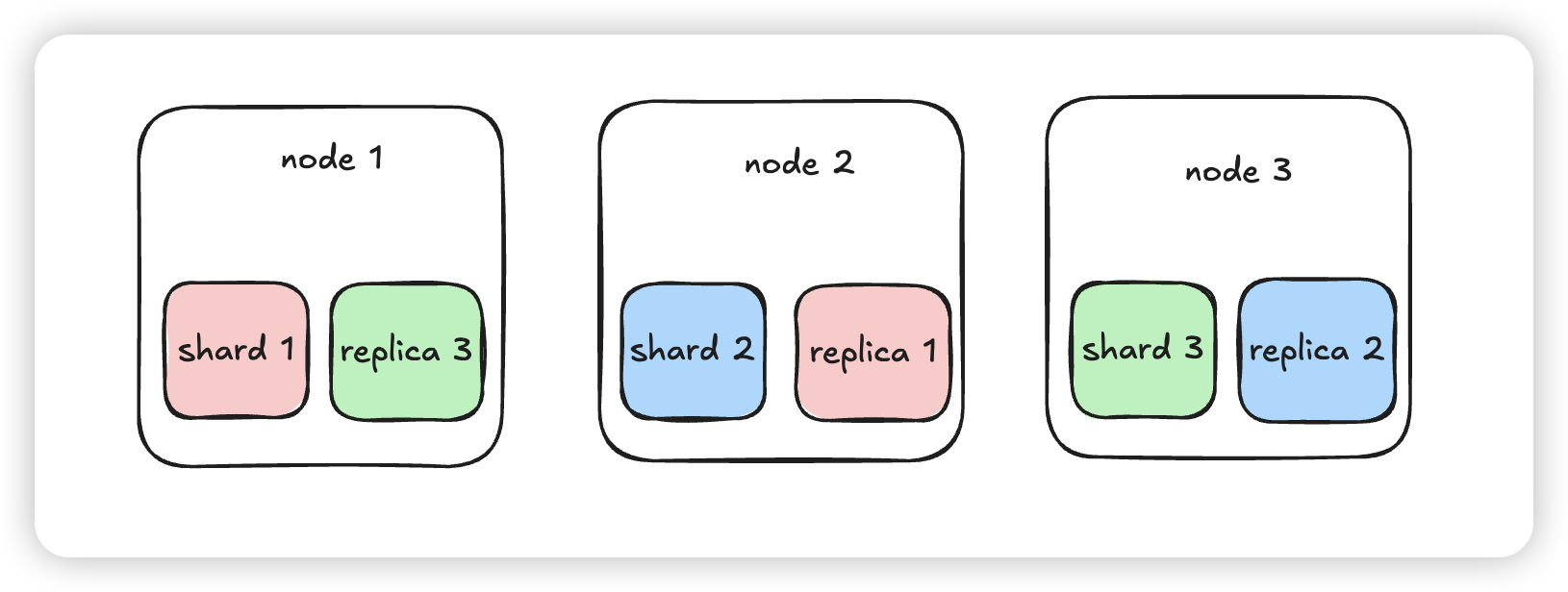 이 때, replica에도 primary shard의 index 정보를 copy하기에 knn index 메모리를 두배로 사용 (alwaysLoadKnnIndex default true)
실제 production 환경에서 총 indexing memory만 15GB 필요
-
Document embedding시 chuncking
- embedding model의 input size 및 맥락을 위해 문서를 쪼개는 chunking 과정 진행
- 때문에 하나의 문서당 여러개의 벡터로 표현 → vector 갯수 증가 → 메모리 사용 증가
-
내주 수행할 내용
vectorDB HNSW 인덱싱 메모리 이슈 문제 실험 및 수치화
- HNSW 그래프가 메모리에 상주해야 하는 구조적 특성으로 인한 서비스 상의 문제점 정리
- 예상 시나리오:
- 다수의 샤드/노드에 대용량 벡터 인덱스를 분산 배치했을 때의 메모리 소비 패턴
- 실험 계획:
- 벡터 개수, dimension, 파라미터별 메모리 사용량 및 검색 latency 수치화
- 벡터 수 증가에 따른 메모리 사용량 곡선 도출 (e.g., 1M, 10M, 100M vectors) 해결 방안 서치
- vector qunatization으로 가능한가?
- disk based indexing으로 해결 가능한가?
참고 논문: https://arxiv.org/abs/2405.03267 https://proceedings.neurips.cc/paper_files/paper/2019/file/09853c7fb1d3f8ee67a61b6bf4a7f8e6-Paper.pdf
2주차 (Opensearch load experiment)
질문#1) Milvus를 사용했나요? VM 노드 세개에 deploy를 한 것 같은데, FAISS를 어떻게 사용했는지, 알려주세요.
문서들의 lexcial search도 필요하여, OpenSearch (Elastic Search fork)를 활용했었습니다.
clustering을 통해
- 3 manger nodes(c6g.large.search, 2vCPU, 4GB)
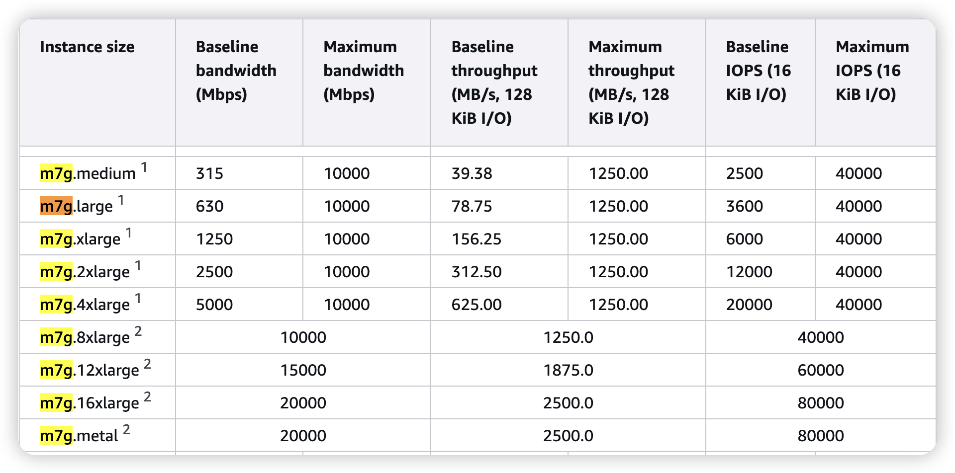
- 3 data nodes(m7g.xlarge.search, 4vcpu, 16GB)
AWS OpenSearch 솔루션으로 해당 cluster 관리를 했습니다.
plugin으로 faiss, lucene, nmslib 등 vector search engine을 지원하여 이 중 faiss를 사용했습니다.
질문#2) Index build 시간도 궁금합니다.
Index를 생성(build)하는 시간 자체는 거의 걸리지 않았습니다.
다만 기존 이미 생성된 Index의 세팅을 변경 시(샤드 개수, hnsw 파라미터 수정)에는 reindex를 진행어야 했고, 이는 기존 index에서 copy하는 방식으로, 같은 수의 insert와 거의 동일한 시간이 걸렸습니다.
질문#3) Index build가 된 이후, CRUD 연산 시간 - Create: 새로운 embedding 추가시 걸리는 시간 - Update: Document가 업데이트 된 경우 embedding이 바뀌면, Index rebuild? 를 하는지, 한다면, 걸리는 시간 - Delete: 위와 동일한 시간
해당 production 환경에 접근이 불가능해서 local에서 재현했습니다.
금주 수행한 내용
vectorDB HNSW 인덱싱 메모리 이슈 문제 실험 및 수치화
HNSW 그래프가 메모리에 상주해야 하는 구조적 특성으로 인한 서비스 상의 문제점 정리
Env
production 환경과 비슷한 local 실험 환경 재구성
OpenSearch cluster (3 node)
- 호스트에 3개의 container로 opensearch cluster 생성
- Host : 11 core, 36GB
- 1.2M document Indexed
Metric
- cpu usage (1분간 점유한 코어 개수 평균)
- virtual memory
- rss (physical memory allocated)
- file IO
Index Create
"embedding": {
          "type": "knn_vector",
          "dimension": 1024,
          "method": {
            "engine": "faiss",
            "space_type": "l2",
            "name": "hnsw",
            "parameters": {
              "ef_construction": 128,
              "m": 16
            }
          }
        },
Document Insert (20만개 삽입)
- 임베딩된 문서를 삽입하는 task 제출 이후 cluster 상태 확인
Search
- 문서 삽입 이후, topk 100 query시에 latency 및 노드 모니터링
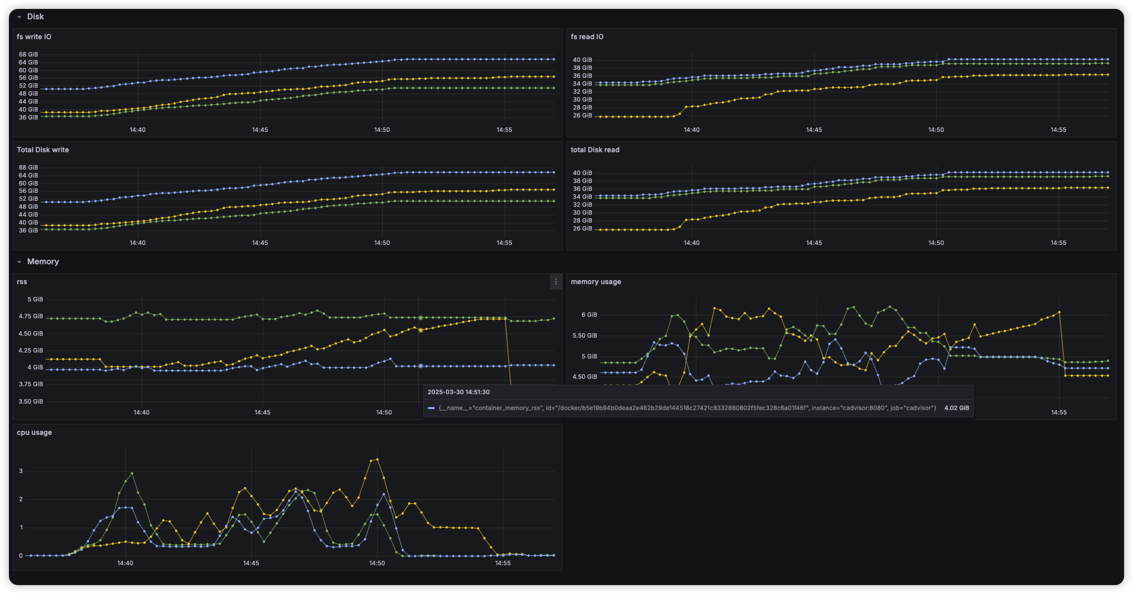
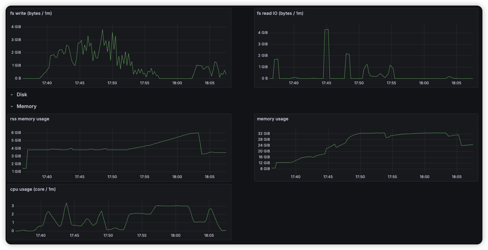
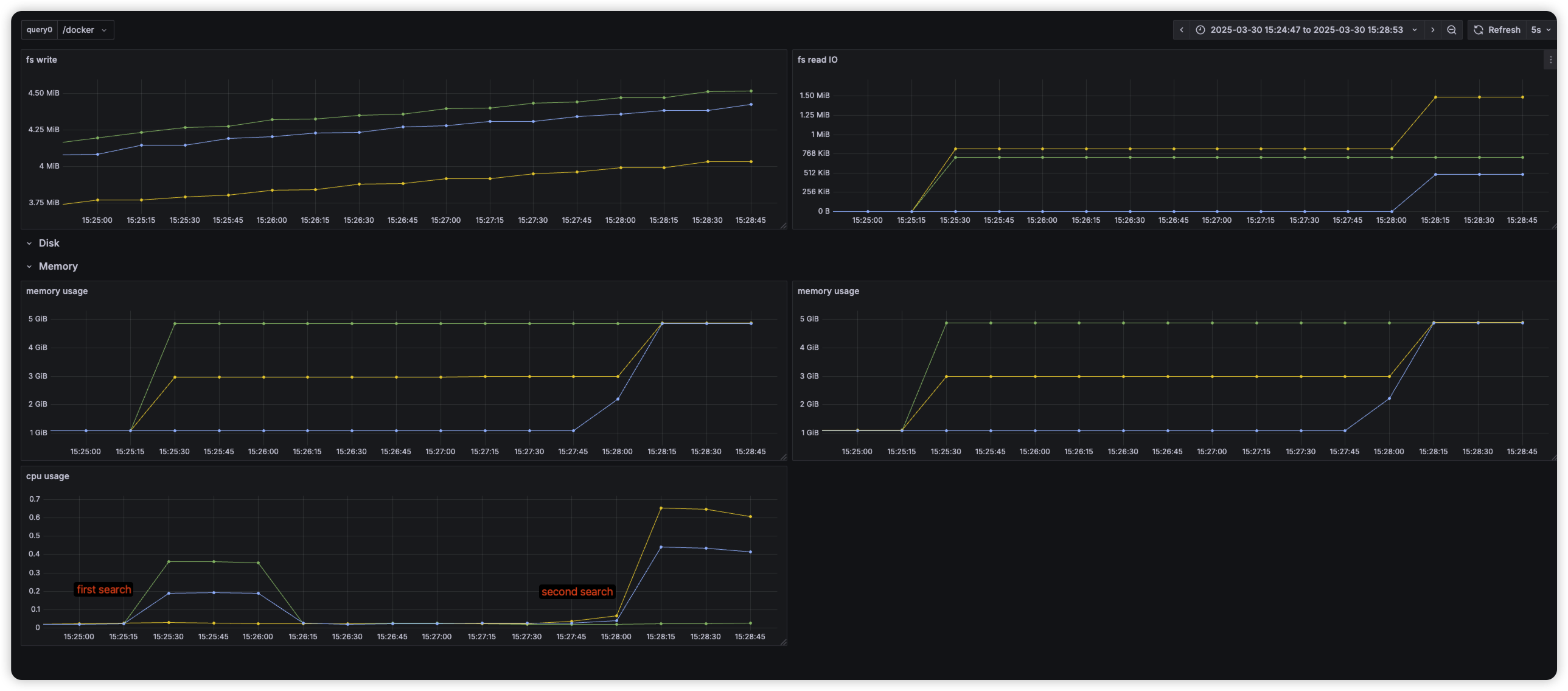 문서 삽입 이후 HNSW 인덱스가 바로 메모리에 올라오지 않고 file 형태로 저장 확인
이후 요청시, memory 올려 놓아 cold start 발생
문서 삽입 이후 HNSW 인덱스가 바로 메모리에 올라오지 않고 file 형태로 저장 확인
이후 요청시, memory 올려 놓아 cold start 발생
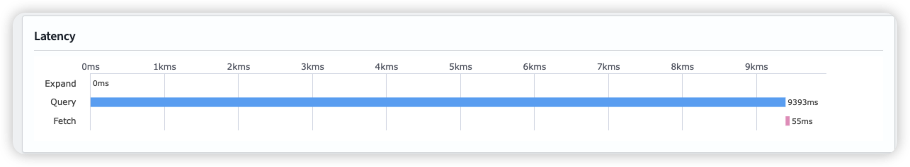
first search latency
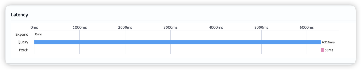
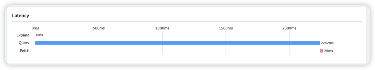
Second Search latency
Warm up
Index에 있는 hnsw graph를 메모리에 올려 놓아, search 요청 시 바로 처리하도록 함
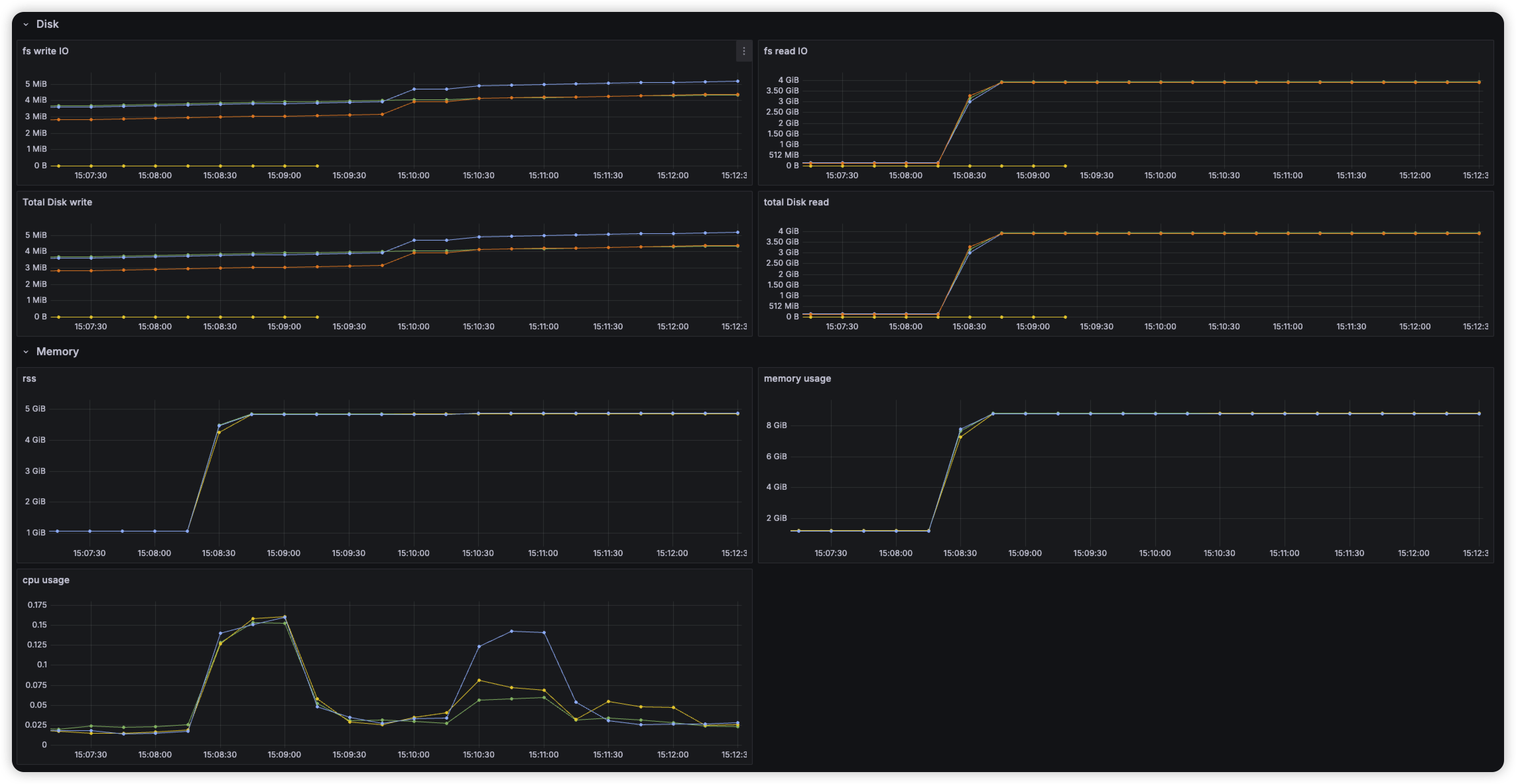
warm-up 요청 시, 노드당 3.5GB의 인덱스를 메모리에 올려놓는 것을 확인
After warm-up
이슈
- 반복적으로 메모리에 index load, store시 JVM GC 작동
2025-03-30 17:41:11 opensearch-node3 | [2025-03-30T08:41:11,213][INFO ][o.o.m.j.JvmGcMonitorService] [opensearch-node3] [gc][130] overhead, spent [708ms] collecting in the last [1.7s]
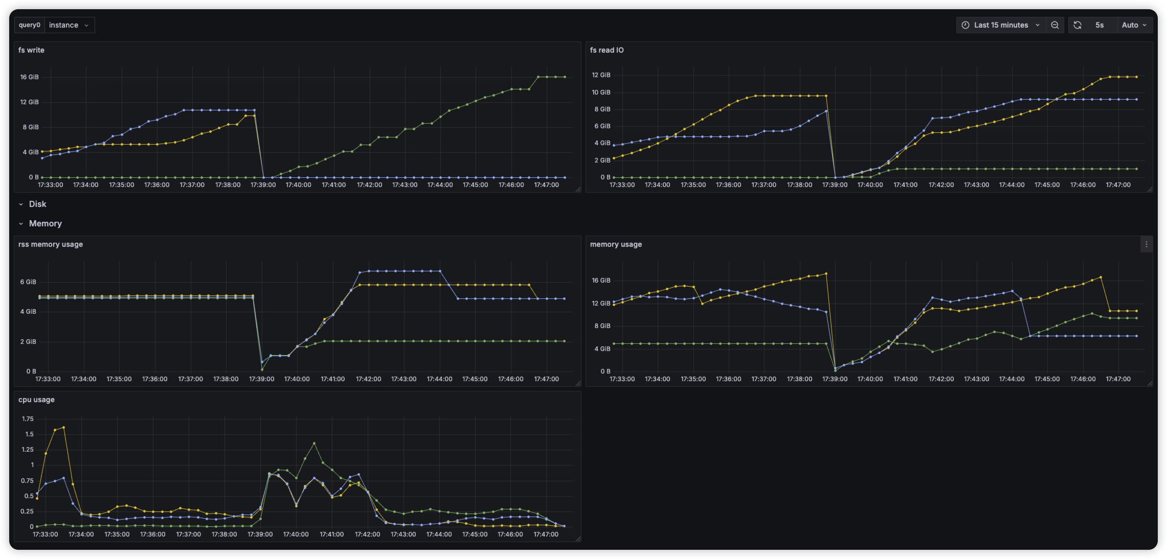
- 샤드 재분배 작업 샤드간 비슷한 크기를 갖도록 유지하는데, node의 상태에 따라 간혹 불균일한 샤드를 갖게될 경우 이를 재할당 함
GET _list/shards/target-index

target-index 0 r STARTED    238002 5.3gb 172.23.0.3 opensearch-node3
target-index 0 p STARTED    238002 5.3gb 172.23.0.5 opensearch-node1
target-index 1 r STARTED    238174 5.3gb 172.23.0.3 opensearch-node3
target-index 1 p STARTED    238174 5.3gb 172.23.0.4 opensearch-node2
target-index 2 r STARTED    238053 5.3gb 172.23.0.3 opensearch-node3
target-index 2 p STARTED    238053 5.3gb 172.23.0.5 opensearch-node1
target-index 3 r STARTED    238743 5.3gb 172.23.0.3 opensearch-node3
target-index 3 p RELOCATING 238743 5.3gb 172.23.0.5 opensearch-node1 -> 172.23.0.4 UnHMdjXFREi63---U6yhEA opensearch-node2
target-index 4 r STARTED    238772 5.3gb 172.23.0.5 opensearch-node1
target-index 4 p STARTED    238772 5.3gb 172.23.0.4 opensearch-node2
target-index 5 p STARTED    239197 5.3gb 172.23.0.5 opensearch-node1
target-index 5 r STARTED    239197 5.3gb 172.23.0.4 opensearch-node2
next_token null
이 때, 많은 File IO 및 메모리 부하 확인
Insight
- local 환경이라 disk → memory로 로드가 빠를텐데, cloud 환경이라면 이과정이 상당히 오래걸리지 않을까?
- cloud 기반 DB들은 대부분 EBS 스토리지를 사용할텐데, 이는 실시간 서비스를 구축하기엔 latency가 너무 길지 않을까?
- 특히나 vector search(HNSW)의 구조상 인덱스에 저장하는 크기가 너무 빠르게 증가함
내주 수행할 내용
- 반복적인 인덱스 memory load, store이 다른 VectorDB solution(Milvus) 혹은 vector engine(faiss)에도 적용이 되는지 확인
- HNSW를 제외한 다른 ANN 알고리즘에서 해당 문제를 어떻게 접근하는지 확인
- disk based indexing으로 해결 가능한가? https://arxiv.org/abs/2310.00402
3주차 (OpenSearch inner HNSW indexing)
금주 수행한 내용
OpenSearch에서 Indexing시 메모리 이슈 수치화
production 환경에서 발생했던 이슈를 local에서 재현하며 문제점 확인
- 인덱싱 시, 많은 Disk I/O 발생 확인
인메모리 구조의 HNSW 알고리즘 특성상 Search, Indexing 시 메모리에 그래프 자료구조를 모두 올려야 함
OpenSearch의 경우 JNI를 통해 C++로 구현된 faiss 이용 faiss에는 HNSW 인덱스를 file로 write,read하는 Interface 제공
void write_index(const Index* idx, const char* fname, int io_flags = 0);
void write_index(const Index* idx, FILE* f, int io_flags = 0);
void write_index(const Index* idx, IOWriter* writer, int io_flags = 0);
해당 인터페이스를 통해 많은 File IO가 발생하는 것을 확인
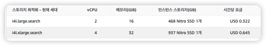
- 해당 실험은 볼륨을 MVME으로 사용
클라우드 서비스에서의 VectorDB
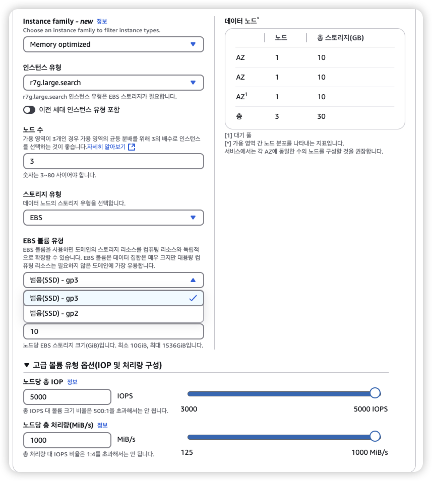
OpenSearch Instance에 AWS EBS를 볼륨을 붙여서 문서들과 Index를 함께 disk에 저장
- 문서 : 큰 용량, 적은 확률로 접근
- 인덱스 : 상대적으로 작은 용량, 잦은 memory to disk load, flush → 병목 예상가능
이를 분리하여 인덱스만 NVME 에 저장하는 것은 불가능
그렇다고 EBS가 아닌, io1 를 붙여서 문서와 함께 저장하는 것은 비효율적임
내주 수행할 내용
- cloud disk latency 실험
- 볼륨으로 많이 사용되는 AWS EBS gp3가 정말 병목일까?
- 가설 확인
- 인덱스를 disk에 바로 write하지 않고
redis같은 별도의 캐시 저장소를 둔다면?- index를 segment로 나눠서, key-value store를 따로 둔다면?
- DPU를 통해서 file cache처럼 쓸 수 있지 않을까?
- 인덱스를 disk에 바로 write하지 않고
4주차 (Faiss HNSW indexing)
금주 수행한 내용
HNSW 인덱스의 메모리 사용 최적화 가능성 탐색
벤치마크
OpenSearch의 HNSW 인덱싱 문제를 확인하기 위해 OpenSearch의 KNN 인덱싱에 활용되는 FAISS을 통해 디스크별 인덱스 생성 및 검색, 저장/복원 과정의 성능평가
#include <iostream>
#include <vector>
#include <chrono>
#include <cstdio>
#include <faiss/IndexHNSW.h>
#include <faiss/index_io.h>

int main() {
    int d = 1024;       // 벡터 차원
    int nb = 50000;    // 벡터 수
    int k = 5;          // topk
    const char* index_file = "hnsw_index.faiss";

    // 벡터 생성
    std::vector<float> xb(d * nb);
    for (int i = 0; i < nb * d; i++) {
        xb[i] = static_cast<float>(drand48());
    }

    int M = 16;
    faiss::IndexHNSWFlat index(d, M);
    index.hnsw.efConstruction = 20;

    // Indexing (add) 시간 측정
    auto start_add = std::chrono::high_resolution_clock::now();
    index.add(nb, xb.data());
    auto end_add = std::chrono::high_resolution_clock::now();
    std::chrono::duration<double> add_time = end_add - start_add;
    std::cout << "[Timing] Indexing (add): " << add_time.count() << " seconds" << std::endl;

    // Write (저장) 시간 측정
    auto start_write = std::chrono::high_resolution_clock::now();
    faiss::write_index(&index, index_file);
    auto end_write = std::chrono::high_resolution_clock::now();
    std::chrono::duration<double> write_time = end_write - start_write;
    std::cout << "[Timing] File write: " << write_time.count() << " seconds" << std::endl;

    // Read (불러오기) 시간 측정
    auto start_read = std::chrono::high_resolution_clock::now();
    faiss::Index* loaded_index = faiss::read_index(index_file);
    auto end_read = std::chrono::high_resolution_clock::now();
    std::chrono::duration<double> read_time = end_read - start_read;
    std::cout << "[Timing] File read: " << read_time.count() << " seconds" << std::endl;

    // 검색용 쿼리 벡터 준비
    std::vector<float> xq(xb.begin(), xb.begin() + d);
    std::vector<faiss::idx_t> I(k);
    std::vector<float> D(k);

    // Search 시간 측정
    auto start_search = std::chrono::high_resolution_clock::now();
    loaded_index->search(1, xq.data(), k, D.data(), I.data());
    auto end_search = std::chrono::high_resolution_clock::now();
    std::chrono::duration<double> search_time = end_search - start_search;
    std::cout << "[Timing] Search: " << search_time.count() << " seconds" << std::endl;

    delete loaded_index;
    return 0;
}
- NVME
[Timing] Indexing (add): 4.81904 seconds
[Timing] File write: 0.006278 seconds
[Timing] File read: 0.00842783 seconds
[Timing] Search: 0.000259917 seconds
- RAMDISK
[Timing] Indexing (add): 4.7268 seconds
[Timing] File write: 0.0151112 seconds
[Timing] File read: 0.00790933 seconds
[Timing] Search: 0.000222875 seconds
- USB
[Timing] Indexing (add): 4.83174 seconds
[Timing] File write: 5.10055 seconds
[Timing] File read: 0.00938633 seconds
[Timing] Search: 0.000263083 seconds
적당한 지연이 있는 디스크를 통해 추후 재실험 예정
인사이트
- 초기 인덱싱에서는 오히려 file write, read 보다 인덱싱 자체가 지연 → 추후 데이터 쌓아서 실험
- faiss가 제공하는 인덱스 저장 방식은 file기반인데, 이걸 메모리 기반 DB에 저장하면 안될까?
- LSM tree DB 기반으로 메모리에 중간 stage를 두어 write latency와 flush 효율 개선하면?
- HNSW의 마지막 layer는 노드 수가 많아, 이를 클러스터 기반(IVF) segment 파일로 나누어 저장하면 prefetch 및 partial load가 개선되지 않을까?
- HNSW을 알고리즘을 변경하여 메모리 이슈를 해결한 연구는 없을까?
- DiskANN, IVFPQ
차주 수행할 내용
- cloud disk latency 실험
- aws or gcp cloud 계정이 별도로 없어, 추후 확인
- 해당 메모리 이슈를 해결한 DiskANN 알고리즘 리뷰
5주차 (DiskANN review)
금주 수행한 내용
DiskANN 논문 리뷰
motivation
- ANN의 목표인 정확도 (recall), 지연시간 (latency), 적은 메모리 사용량을 모두 만족하기 위한 방법 제시
- HNSW은 높은 recall을 보여주지만, 메모리 상주 이슈로 대규모 데이터셋 처리엔 한계
DiskANN
- 원본 벡터(full-precision)와 neighbor ID list는 SSD에 저장, 압축된 벡터(product quantization)은 메모리에 저장
- 각 노드의 데이터는 SSD의 4KB 블록 단위로 저장되며,
하나의 블록(4kb)에 full-precision 벡터와 이웃 리스트가 함께 포함되도록 구성 - 이 구조는 디스크 접근 시 한 번의 I/O로 필요한 모든 정보를 가져올 수 있게 하여 latency를 최소화함
- 탐색 depths를 줄여 disk 접근을 적게 만듦
Vamana 알고리즘
- 그래프 기반 인덱싱 방식으로, 탐색 직경을 줄이기 위한 α-parameter 기반 pruning 전략 사용
- 전체 데이터셋에 대해 두 번의 패스를 진행하여 탐색 품질 개선
- 첫 번째 패스: α=1로 기본 연결 생성
- 두 번째 패스: α>1 (e.g., 1.2)로 long-range edge 추가
- 인접 노드 선택 시, 거리 기반이 아니라 α-기반 조건으로 long, diverse connection 확보
- 결과적으로 SSD 기반 탐색에서 필요한 노드 수, 즉 디스크 접근 횟수를 줄이도록 설계됨
Indexing
memory
- 모든 벡터들을 압축한 상태로 저장
- Product Quantization, which encodes the data and query points into short codes (e.g., 32 bytes per data point)
disk
[ disk block (4KB aligned) ]
┌────────────────────────────────────────────┐
│ Full-precision vector (e.g., 128D float32) │  → 128 * 4B = 512B
├────────────────────────────────────────────┤
│ Neighbor list (R개 노드 ID)                  │ → R * 4B (e.g., R=64 → 256B)
├────────────────────────────────────────────┤
│ Padding / reserved                         │  → 나머지 공간 (alignment 맞춤)
└────────────────────────────────────────────┘
Search
xq: 쿼리 벡터L: 후보 리스트 크기W: Beam width (한 번에 SSD에서 읽을 노드 수)k: 찾고자 하는 최근접 이웃 수
입력: 쿼리 xq, 시작 노드 s, 후보 리스트 크기 L, Beam Width W

1. 초기화:
   - 후보 리스트 L ← {s}
   - 방문한 노드 집합 V ← ∅

2. 반복:
   - 아직 방문 안한 후보 중 쿼리와 가장 가까운 W개 노드를 SSD에서 한 번에 읽음
   - 읽은 각 노드의 이웃 리스트 + full-precision 벡터 함께 가져옴
   - 이웃 노드들의 PQ 벡터를 이용해 거리 계산 후, 후보 리스트에 추가
   - 방문 노드 집합 V에 읽은 노드 추가

3. 후보 리스트가 충분히 수렴하거나 max hops에 도달하면 종료

4. 최종 후보 중 full-precision 벡터로 거리 다시 계산 → top-K 결과 반환
평가
환경 • z840: a bare-metal mid-range workstation with dual Xeon E5-2620v4s (16 cores), 64GB DDR4 RAM, and two Samsung 960 EVO 1TB SSDs in RAID-0 configuration.
• M64-32ms: a virtual machine with dual Xeon E7-8890v3s (32-vCPUs) with 1792GB DDR3 RAM that we use to build a one-shot in-memory index for billion point datasets.
| 데이터셋 | 차원 수 |
|---|---|
| SIFT | 128D |
| DEEP | 96D |
| GIST | 960D |
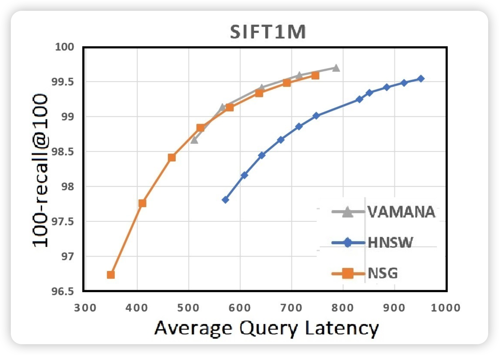
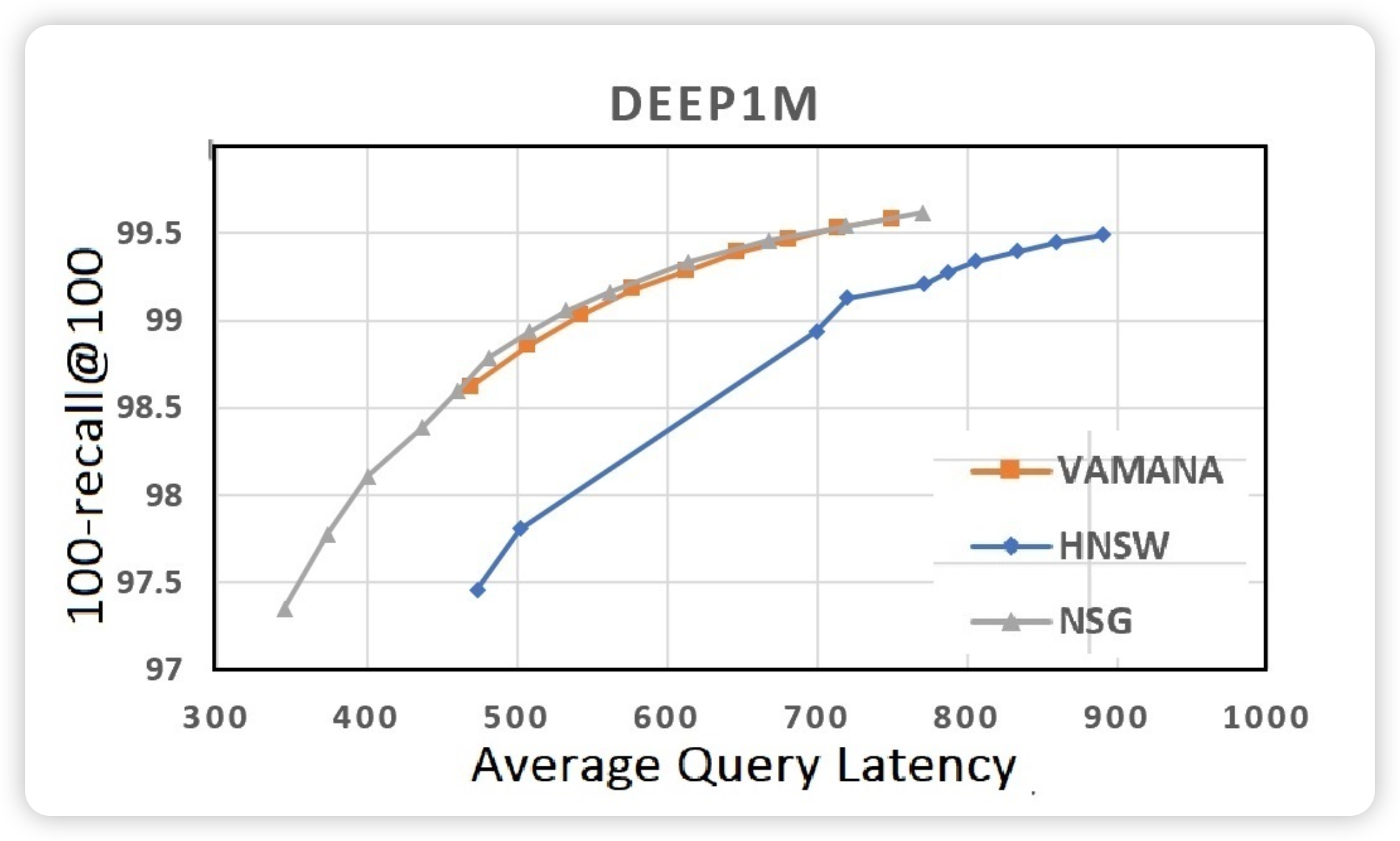
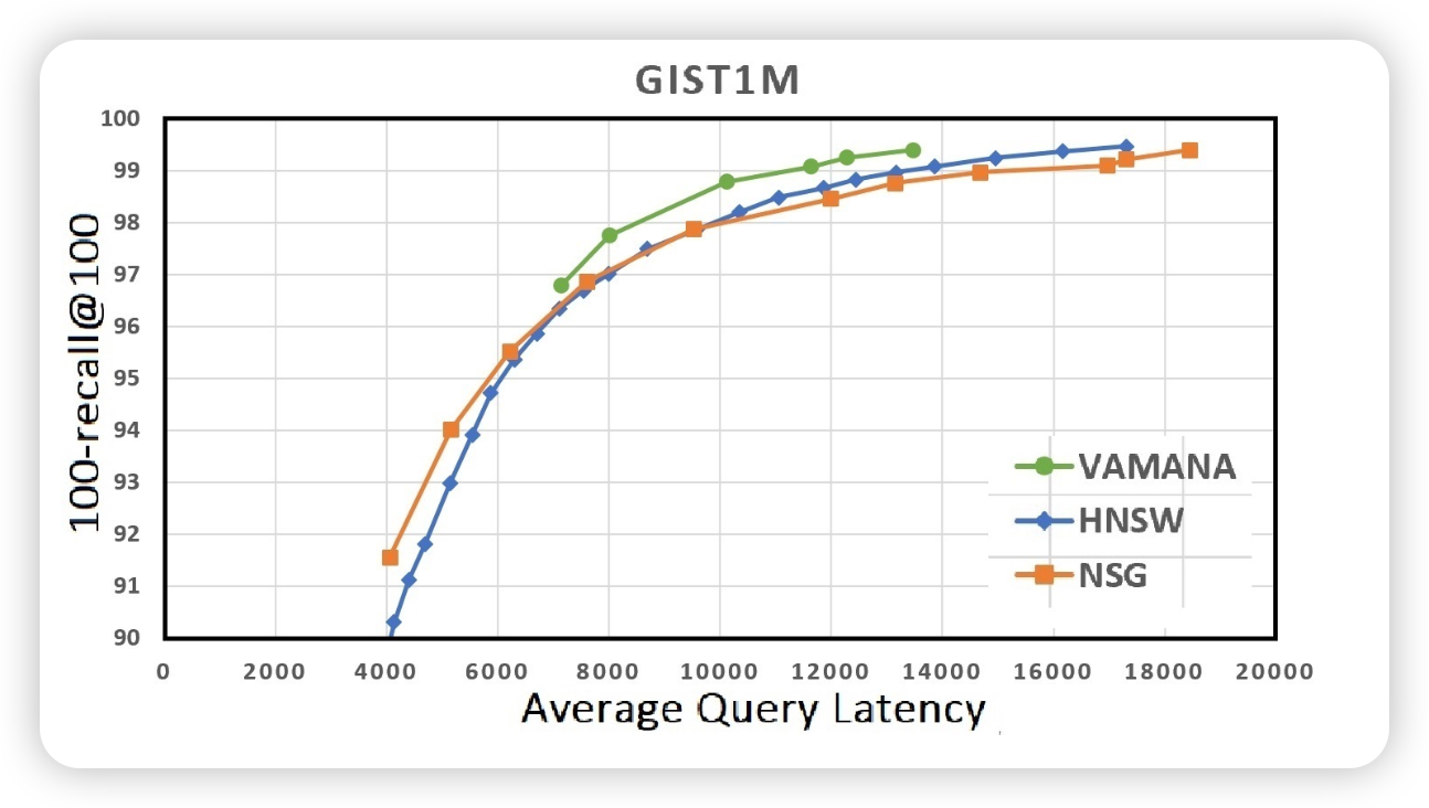
recall & latency
100-recall@100: Top-100 중 맞춘 비율
| 데이터셋 | 알고리즘 | 100-recall@100 | Latency (μs) |
|---|---|---|---|
| SIFT1M | Vamana | 99.7% | 500~700μs |
| HNSW | ~99.3% | 600~900μs | |
| NSG | ~99.5% | 400~700μs | |
| GIST1M | Vamana | ~99.2% | 6000~15000μs |
| HNSW | ~98.8% | 5000~18000μs | |
| NSG | ~98.7% | 5000~16000μs | |
| DEEP1M | Vamana | 99.5% | 400~700μs |
| HNSW | ~98.3% | 400~900μs | |
| NSG | ~99.4% | 400~750μs |
memory footprint
| 데이터셋 | 차원 수 | 벡터 수 | 알고리즘 | Latency (ms) | 메모리 사용량 | 디스크 사용량 |
|---|---|---|---|---|---|---|
| SIFT1B | 128D | 1B | DiskANN | < 5ms | ≤ 64GB (merged index 기준) | 348GB (SSD) |
| HNSW | 1~2ms (RAM) | 250GB ~ 1TB 이상 예상 | RAM-only |
“DiskANN can index and serve a billion point dataset in 100s of dimensions on a workstation with 64GB RAM…”
“DiskANN serves 5−10x more points per node compared to state-of-the-art graph-based methods such as HNSW and NSG.”
한계
- 원본 벡터 + 인접 리스트를 4kb 디스크블록에 저장하면, 1024 차원(4kb)이상 벡터는 저장이 안되지 않나?
- 실험 데이터셋 중 가장 고차원인 GIST1M (960D)까지만 사용됨
- 1024D 이상 벡터는 벡터 크기만으로도 4KB → 이웃 리스트 포함 불가
- RAG시스템에서 활용할 고차원 벡터 인덱싱으로 사용하기에 적합한가?
- OpenAI embedding model: the length of the embedding vector is
1536fortext-embedding-3-smallor3072fortext-embedding-3-large - DiskANN 기본 설계로는 저장 불가능 → PQ 압축 필요
- OpenAI embedding model: the length of the embedding vector is
- 실제 구현을 확인해보면 1024차원이 넘으면 압축해서 disk에 저장하도록 옵션 제공 → recall 하락
DiskANN parameter PQ_disk_bytes (default is 0): Use 0 to store uncompressed data on SSD. This allows the index to asymptote to 100% recall. If your vectors are too large to store in SSD, this parameter provides the option to compress the vectors using PQ for storing on SSD. This will trade off recall. You would also want this to be greater than the number of bytes used for the PQ compressed data stored in-memory
차주 수행할 내용
- product quantization으로 고차원 벡터에서도 recall이 유지되는지 실험
- HNSW vs DiskANN
- faiss
IndexHNSWPQvsIndexHNSWFlat
6주차 (Proposal presentation)
1. Introduction — Why VectorDB Matters
1.2 Vector Dataset Size
VectorDB usage in RAG system. Assumption knowledge base like wikipedia
| Category | Calculation | Result |
|---|---|---|
| Short articles (90%) | 6.7M × 0.9 × 1 vector | 6.03M vectors |
| Long articles (10%) | 6.7M × 0.1 × 2.5 vectors | 1.675M vectors |
| Total | 6.03M + 1.675M | 7.705M vectors |
-
Assumes no chunking; each document up to 8192 tokens (OpenAI embedding model limit).
-
Using 1,024-dimensional embeddings, each vector occupies 4 KB (float32).
-
Storage requirement for raw vectors:
1.3 Cloud Reality Check
| Dimension | Traditional Assumption | Cloud Reality (256 GB RAM Instance) |
|---|---|---|
| Storage | Local NVMe (μs latency) | Network-attached EBS / persistent disks (ms latency) |
| Memory | 512 GB–1 TB RAM affordable once | RAM constrained to 256 GB, high per-hour costs |
| Scaling | Single rack, static provisioning | Elastic scaling and auto-recovery expected |
Key takeaway:
Existing vector search engines, optimized for abundant RAM and fast local disks, face significant cost and latency constraints in 256 GB cloud environments.
2. HNSW Recap — Strengths & Inner Workings
2.1 Concept
- HNSW (Hierarchical Navigable Small-World Graph) builds multi-layer graphs:
- Sparse upper layers
- Dense base layer
- Greedy graph traversal from top layers to bottom achieves efficient approximate search.
2.2 Why It Shines
| Property | Effect |
|---|---|
| Logarithmic search paths | Sub-millisecond CPU even at large scale |
| Strong graph locality | High recall (> 0.98) without exhaustive scanning |
| Purely in-memory design | No decompression or disk access during search |
2.3 Internal Parameters Cheat-Sheet
| Symbol | Typical Range | Purpose |
|---|---|---|
| M | 16–32 | Max neighbors per node |
| efConstruction | 200–400 | Graph construction quality trade-off |
| efSearch | 32–128 | Search recall vs latency |
3. HNSW Cloud Pain-Points
3.1 Full-RAM Requirement
Memory footprint estimation (float32 format):
Example for Wikipedia-scale:
-
7.7M vectors × 1024 dimensions → ~30.8 GB raw vectors
-
+6.4 GB for graph structure (M=32)
-
⇒ ~37.2 GB total RAM required
-
In practice, indexing additionally requires ~1.5–2× RAM due to working buffers, meaning peak RAM usage can reach 60–80 GB.
3.2 Random Access Pattern
- HNSW graph traversal is non-sequential.
- Each memory miss under mmap triggers a page fault, causing 4–64 KB random reads on network-attached EBS volumes.
- Empirical results show:
- 1000 random 4 KB reads on AWS gp3 ≈ 10 ms p99 latency (vs <200 μs on NVMe).
Random disk I/O dominates latency unless the full graph resides in memory.
3.3 Cost Explosion
| Instance | RAM Size | On-demand Cost (2025 AWS) |
|---|---|---|
| r6i.2xlarge | 64 GB | $340/month |
| r6i.8xlarge | 256 GB | $1,350–1,600/month |
Observation:
Even with 256 GB RAM instances, full in-memory indexing and search is feasible only for mid-scale datasets (e.g., ~7–25M vectors at 1024 dims).
Billion-scale indexes become impractical without disk-resident augmentation.
3.4 RAM Overhead During Index Building — FAISS Example
Even if the saved HNSW index is ~37 GB,
index construction phase uses far more RAM.
Breakdown during FAISS HNSW indexing:
| Component | Description | Size Estimate (7.7M vectors) |
|---|---|---|
| Raw vectors (float32) | Full vector set | ~30.8 GB |
| Neighbor links (graph) | HNSW edges | ~6.4 GB |
| Candidate pools and heaps | Search buffers for each thread | 10–20 GB |
| Other malloc overhead | Allocator slack, fragmentation | 10–15 GB |
| Peak RAM usage | - | ~60–80 GB |
Thus, indexing typically demands 1.5–2× the final saved size.
3.5 Key Reasons for High RAM Usage During FAISS HNSW Indexing
- Dynamic Graph Construction:
- Insertions dynamically modify neighbor lists, requiring mutable in-memory structures.
- Multiple Working Buffers:
- Multi-threaded search and insertion use separate candidate buffers and priority queues.
- Low-Latency Full Dataset Access:
- Distance computations must happen in-memory for speed.
- Temporary RAM Peaks:
- RAM usage drops after build but peaks significantly during indexing.
3.6 RAM Budget Estimation for 256 GB Instances
Given 256 GB RAM:
- 50% reserved for raw vectors (~128 GB)
- Remaining accommodates graph links, candidate buffers, and overhead
Thus:
- Each 1024-dim float32 vector (4 KB) means:
- Considering safety margins for working memory:
- Practical safe capacity ≈ 25–28M vectors
| Component | Estimate |
|---|---|
| 1 vector size | 4 KB |
| Max vectors (raw math) | 32M |
| Practical limit | ~25–28M vectors |
Conclusion:
On a 256 GB RAM instance, indexing up to ~28 million 1024-dimensional vectors is feasible with FAISS HNSW.
Beyond that, hybrid disk-resident approaches become necessary.
4. IVF & PQ Quick Glance — Alternative Trade-offs
4.1 IVF (Inverted File Index)
- Clusters vectors using k-means into √N centroids.
- Search probes a small number (nprobe) of closest clusters only.
- Pros: Great memory efficiency; scalable to billions of vectors.
- Cons: Missed centroids lead to sharp recall drops.
4.2 Product Quantization (PQ/OPQ)
- Compresses vectors by dividing into m subspaces, quantizing each separately.
- 16× compression typical (128-dim → 8 bytes).
- Pros: Massive memory savings.
- Cons: Approximate distances introduce errors; decoder overhead (~50–100 ns per comparison).
4.3 Why IVF-PQ Doesn’t Fully Replace HNSW
- Even optimized IVF-PQ setups achieve only 0.92–0.95 recall, falling short of HNSW (~0.98+).
- Retrieval error can propagate, degrading downstream tasks like answer generation in RAG systems.
5. DiskANN — What It Solved
5.1 Core Idea
- Move most of the vector data and graph structure to SSD, leaving only entry points and coarse metadata in RAM.
- Layout vectors into 4 KB blocks sorted by node ID for sequential access.
- Prefetch relevant blocks during search to minimize random I/O.
5.2 Performance on Local NVMe
| Dataset | RAM Usage | SSD QPS | p99 Latency |
|---|---|---|---|
| 1B vectors (96 dim) | 30 GB (vs 320 GB RAM) | 4000 QPS | ~5 ms |
5.3 Key Techniques
- Block Prefetch Queue: Asynchronously load predicted graph blocks.
- Euclidean Pruning: Skip blocks if current best distance suffices.
- Thread-local Hot Caches: Keep frequently accessed nodes resident.
6. DiskANN Gap in Cloud-Native Environments
6.1 Fixed 4 KB Block Size
- EBS and S3 favor sequential reads ≥64 KB.
- 4 KB blocks cause excessive fragmentation and IOPS throttling in cloud disks.
6.2 Blind Prefetch Strategy
- Uniform priority prefetch without IOPS-aware scheduling leads to prefetch congestion.
6.3 Missing Compression Path
- Raw float32 vectors occupy large storage.
- For 10M vectors: ~40 GB storage cost (before replication or backup overhead).
6.4 Single-Node Assumption
- No built-in shard management, replication, or recovery.
- Unsuitable for Kubernetes, multi-zone HA, or dynamic cloud scaling.
6.5 Summary Table
| Aspect | DiskANN (Original) | Cloud-Native Requirement |
|---|---|---|
| Block Size | 4 KB fixed | Tunable (≥64 KB) |
| Prefetch Policy | Uniform frontier prefetch | Priority-aware, IOPS-sensitive |
| Deployment Model | Single host | Multi-node sharding + HA |
6.6 Improve DiskANN on Cloud Environment
- DiskANN are optimized prefetch with request small size IO (4kb block size)
- frequent small size IO can be bottleneck on cloud storage like
EBS gp3
- How about bigger block packing to segment?
(example segment)
┌────────────────────────────────────────────┐
│ **Node 1**                                 │
│ Full-precision Vector (128D float32)       │ → 512B
│ Neighbor List (R=64, Node IDs)             │ → 256B
│ Padding / Reserved Space                   │ → 256B (alignment to 1KB)
├────────────────────────────────────────────┤
│ **Node 2**                                 │
│ Full-precision Vector (128D float32)       │ → 512B
│ Neighbor List (R=64, Node IDs)             │ → 256B
│ Padding / Reserved Space                   │ → 256B (alignment to 1KB)
├────────────────────────────────────────────┤
│ **Node 3**                                 │
│ Full-precision Vector (128D float32)       │ → 512B
│ Neighbor List (R=64, Node IDs)             │ → 256B
│ Padding / Reserved Space                   │ → 256B (alignment to 1KB)
├────────────────────────────────────────────┤
│ ... (More Nodes)                           │
├────────────────────────────────────────────┤
│ **Metadata**                               │
│ Node IDs included in segment               │ → e.g., {Node 1, Node 2, Node 3..}
│ Segment Offset Map                         │ → {Node 1 @ 0B, Node 2 @ 1KB, ...}
│ Checksum / Validation Data                 │ → For data integrity
│ Reserved Space for future use              │
└────────────────────────────────────────────┘